YOLOv3 Object Detection
Author: Shahidul Islam
Created: 08 Dec, 2020
Last Updated: 11 Feb, 2021
Last Updated: 11 Feb, 2021
Object detection is a task that involves identifying the presence, location and type of one or more objects in an image. Yolo which stands for ‘you only look once’ is an object detector model that uses deep convolutional neural network. In this blog, we will discuss YOLOv3, a variant of the original YOLO model that achieves near state-of-the-art(SOTA) result. YOLOv3 can perform object detection in real-time.
Model Overview:
Basically YOLOv3 model has two different parts:
1. Feature extraction.
2. Bounding box prediction.
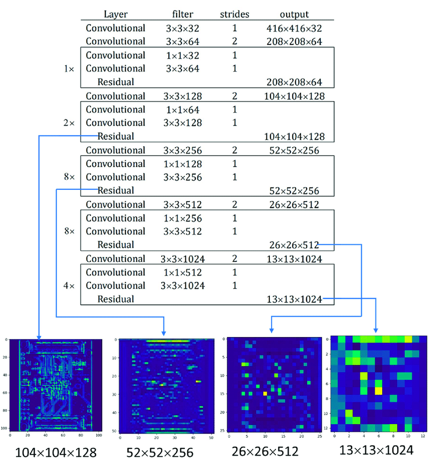
Feature extraction: Yolov3 uses a larger network to perform feature extraction than yolov2. This model is known as DARKNET-53 which has 53 convolution layers with residual connections. We ignore the last three layers of darknet-53 (avgpool layer, fc layer, softmax layer) as these layers are mainly used for image classification. In this object detection task, we are using darknet-53 only to extract image features so these three layers will not be needed.
Darknet-53 uses a new kind of block called Residual Block. Deep neural networks are difficult to train. With the depth increasing, sometimes network accuracy gets saturated which leads to higher training error. To solve this problem residual block was introduced. The architectural difference between normal convolution block and the residual block is the addition of skip connection. Skip connection carries the input to the deeper layers.
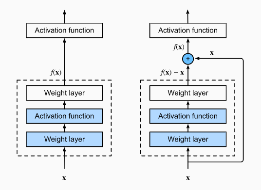
Let’s denote the input by \(x\) and The desired mapping that we want to obtain by learning is \(F(x)\). On the left of the above figure, the dotted box directly learns the mapping \(F(x)\). The right side of the above figure shows how the residual block looks like. The dotted box portion learns a slightly different mapping, \(F(x)-x\). This mapping is easier to learn. To obtain the actual mapping \(F(x)\), the input \(x\) get added with the mapping \(F(x)-x\). The solid line that adds the input \(x\) to the mapping is called a residual connection or shortcut connection. The addition of \(x\) acts like a residual, hence the name ‘residual block’.
Here is the implementation of darknet-53 in python.
def residual_block(input_layer, input_channel, filter_num1, filter_num2):
    short_cut = input_layer
    conv = convolutional(input_layer, filters_shape=(1, 1, input_channel, filter_num1))
    conv = convolutional(conv       , filters_shape=(3, 3, filter_num1,   filter_num2))
    residual_output = short_cut + conv
    return residual_output

def darknet53(input_data, training=False): #python implementation of darknet-53
    input_data = convolutional(input_data, (3, 3,  3,  32))
    input_data = convolutional(input_data, (3, 3, 32,  64), downsample=True)

    for i in range(1):
        input_data = residual_block(input_data,  64,  32, 64)

    input_data = convolutional(input_data, (3, 3,  64, 128), downsample=True)

    for i in range(2):
        input_data = residual_block(input_data, 128,  64, 128)

    input_data = convolutional(input_data, (3, 3, 128, 256), downsample=True)

    for i in range(8):
        input_data = residual_block(input_data, 256, 128, 256)

    route_1 = input_data
    input_data = convolutional(input_data, (3, 3, 256, 512), downsample=True)

    for i in range(8):
        input_data = residual_block(input_data, 512, 256, 512)

    route_2 = input_data
    input_data = convolutional(input_data, (3, 3, 512, 1024), downsample=True)

    for i in range(4):
        input_data = residual_block(input_data, 1024, 512, 1024)

    return route_1, route_2, input_data
Bounding Box Prediction: In the prediction part, the network uses convolution layer, upsample layer, skip connection and convolution layer with stride 2 as downsample layer. We don’t use any kind of pooling layer to downsample the input image as the pooling layer losses more low-level features from the input image.
This network predicts bounding box on downsampled images for fast real-time prediction. We downsample image by a factor, called stride. So stride of the network is equal to the factor by which the output layer is smaller than the input image. YOLOv3 uses three different strides (8, 16, 32). So if the size of the input image is \(416 \times 416\) (without color channel), then the ouput tensors would be \(52\times52\), \(26\times26\), \(13\times13\).
See the yolov3 architecture below for better understanding.
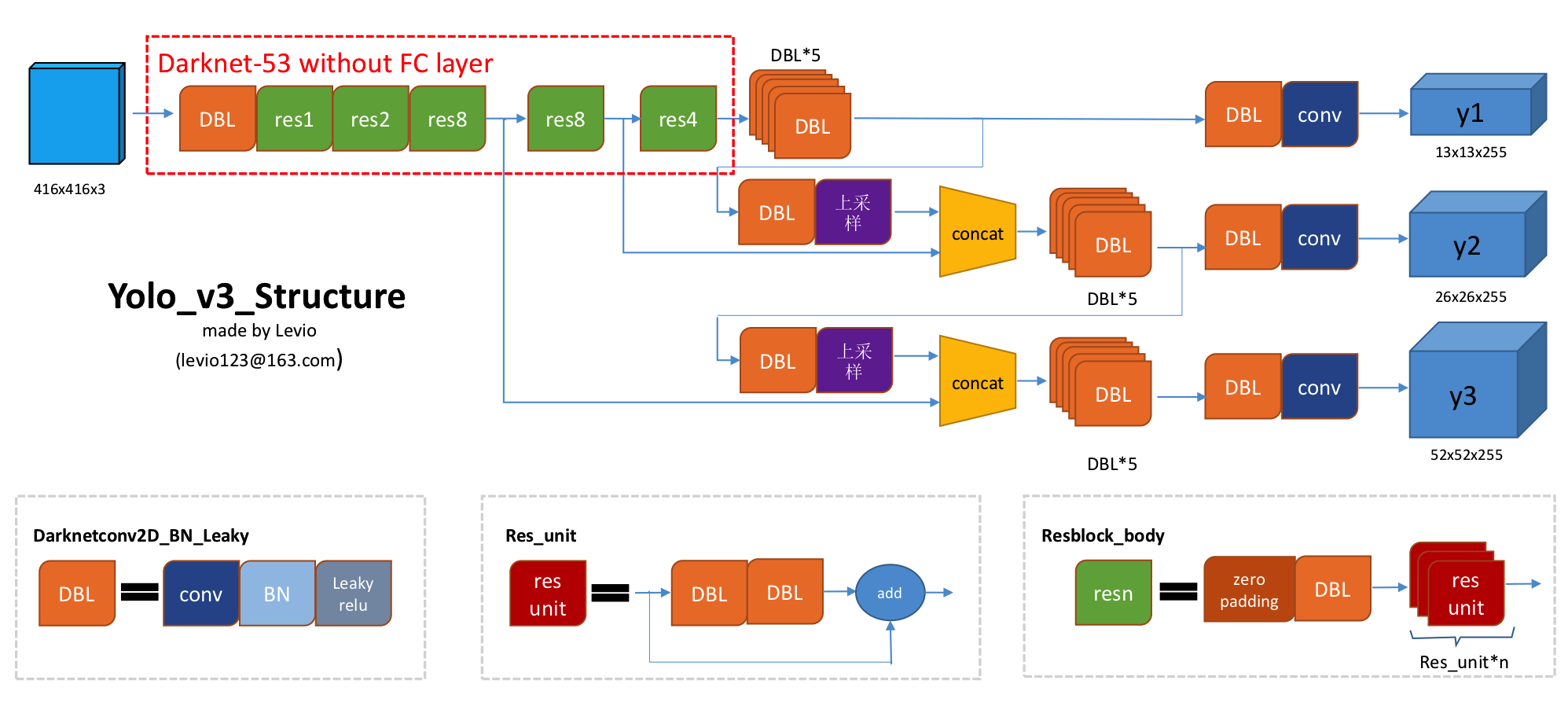
We can see that the network uses three different branches from the darknet-53 model. We add some convolution layer after the last layer of the darknet-53 model and get the first output layer \(y1\). This layer is 32 times smaller than the actual input image. Later we’ll discuss the dimension of output layers(\(y1\), \(y2\), \(y3\)). Next we upsample the layer 2times and concatenate with the second output layer of darknet-53. After adding some convolution layers, we get the output layer \(y2\). By this similar fashion, we also get the output layer \(y3\).
The readers might not understand why we are detecting on three different levels. The answer to this question is that three-level detection helps YOLOv3 detects different size objects more accurately. \(y1\) layer makes the output 32 times smaller than the actual image, \(y2\) makes 16 times smaller and \(y3\) makes 8 times smaller. So large objects get detected more frequently on layer \(y1\), medium size object on layer \(y2\) and small objects on layer \(y3\). This three-layer detection technique helps yolov3 to get better detection than previous variants.
Here is the code of YOLOv3 model.
def YOLOv3(input_layer, NUM_CLASS, training=False): #This function returns output layers of YOLOv3 model
    # After the input layer enters the Darknet-53 network, we get three branches
    route_1, route_2, conv = darknet53(input_layer, training)

    conv = convolutional(conv, (1, 1, 1024,  512))
    conv = convolutional(conv, (3, 3,  512, 1024))
    conv = convolutional(conv, (1, 1, 1024,  512))
    conv = convolutional(conv, (3, 3,  512, 1024))
    conv = convolutional(conv, (1, 1, 1024,  512))
    conv_lobj_branch = convolutional(conv, (3, 3, 512, 1024))

    # conv_lbbox is used to predict large-sized objects , Shape = [None, 13, 13, 255]
    conv_lbbox = convolutional(conv_lobj_branch, (1, 1, 1024, 3*(NUM_CLASS + 5)), activate=False, bn=False)

    conv = convolutional(conv, (1, 1,  512,  256))
    # upsample here uses the nearest neighbor interpolation method, which has the advantage that the
    # upsampling process does not need to learn, thereby reducing the network parameter
    conv = upsample(conv)

    conv = tf.concat([conv, route_2], axis=-1)
    conv = convolutional(conv, (1, 1, 768, 256))
    conv = convolutional(conv, (3, 3, 256, 512))
    conv = convolutional(conv, (1, 1, 512, 256))
    conv = convolutional(conv, (3, 3, 256, 512))
    conv = convolutional(conv, (1, 1, 512, 256))
    conv_mobj_branch = convolutional(conv, (3, 3, 256, 512))

    # conv_mbbox is used to predict medium-sized objects, shape = [None, 26, 26, 255]
    conv_mbbox = convolutional(conv_mobj_branch, (1, 1, 512, 3*(NUM_CLASS + 5)), activate=False, bn=False)

    conv = convolutional(conv, (1, 1, 256, 128))
    conv = upsample(conv)

    conv = tf.concat([conv, route_1], axis=-1)
    conv = convolutional(conv, (1, 1, 384, 128))
    conv = convolutional(conv, (3, 3, 128, 256))
    conv = convolutional(conv, (1, 1, 256, 128))
    conv = convolutional(conv, (3, 3, 128, 256))
    conv = convolutional(conv, (1, 1, 256, 128))
    conv_sobj_branch = convolutional(conv, (3, 3, 128, 256))

    # conv_sbbox is used to predict small size objects, shape = [None, 52, 52, 255]
    conv_sbbox = convolutional(conv_sobj_branch, (1, 1, 256, 3*(NUM_CLASS +5)), activate=False, bn=False)

    return [conv_sbbox, conv_mbbox, conv_lbbox]
Output Layer Explanation: As you all know, YOLOv3 predicts bounding boxes in three different scales. In this section, we’ll understand the output layer of this network. Below I have attached an image of output layer \(y1\) (stride 32).
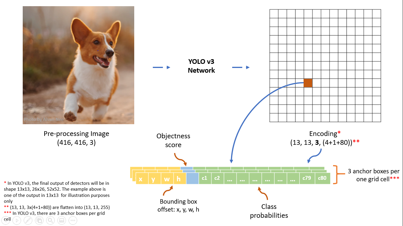
We have downsampled \(416 \times 416\) image to \(13 \times 13\) output tensor. The image has been divided into \(13 \times 13\) blocks and for every block, we predict 3 bounding boxes. So actually for every block, we want to predict three objects whose centers lie in that particular block. For a specific block let’s say for the red block in the above image, we want to detect objects whose centers lie in that block. We can see that this red block predicts 255 values or \(3*85\) (three objects per block). You might wonder why 85 values per bounding box! These values are: 4 bounding box offset, 1 objectness score and 80 class probabilities.
\(x, y\): these two values are the x and y offset of the bounding box this cell predicts.
\(w, h\): These two values are the width and height of the bounding box this cell predicts.
Objectness Score: This score is the confidence score of whether this block contains the center of any object in the actual image. This confidence score does not depend on any specific object.
Class Probabilities: The class probabilities are the probabilities of the detected object belonging to a particular class. In the above image, we assume that our dataset contains 80 different classes. So the class probabilities contain 80 values.
So depth-wise our model predicts \(B * (4+1+C)\) values. Each block predicts \(B\) bounding boxes and every bounding box has \((4+1+C)\) attributes, whice describe the center coordinates, the dimensions, the objectness score and \(C\) class probabilities.
Anchor Box: It might make sense to predict the width and height of the bounding box. But in practice, that leads to unstable gradients during training. So YOLOv3 predicts offsets to pre-defined default bounding boxes, called anchor boxes. YOLOv3 uses different anchors on different scales. YOLOv3 model predicts bounding boxes on three scales and in every scale, three anchors are assigned. So in total, this network has nine anchor boxes. These anchors are taken by running K-means clustering on dataset.
Decode Processing: We have already discussed the output layers of YOLOv3. The output layers predict bounding box coordinates, dimensions, objectness score and class probabilities. As these attributes are just the result of some convolution layers of the network so the values of these attributes can be arbitrarily anything. So these values are transformed by some functions.
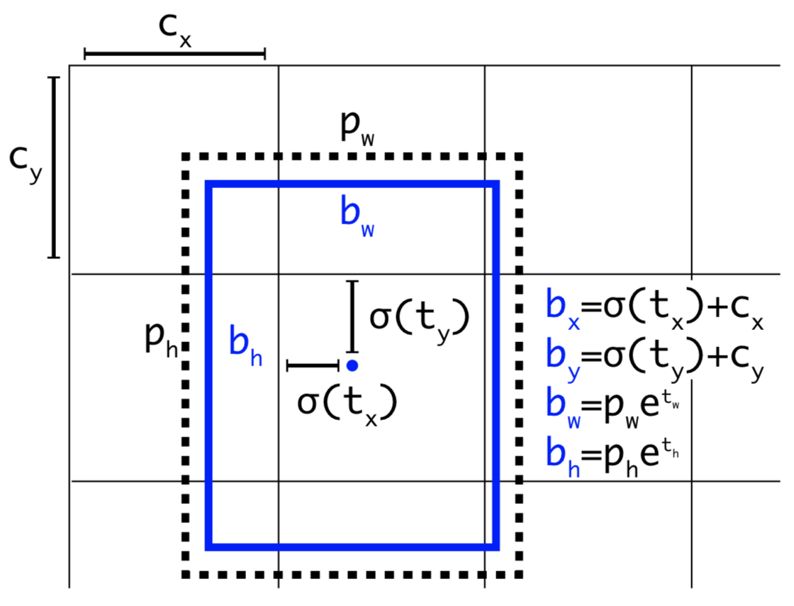
Here \(tx, ty, tw, th\) are the network outputs. \(bx, by, bw, bh\) are the transformed values of \(tx, ty, tw, th\) respectively. \(cx, cy\) are the top-left coordinates of the grid. \(pw, ph\) are the anchor dimensions for this grid.
Center Coordinates: We pass the values of \(tx, ty\) to a sigmoid function. The sigmoid function converts the values between 0 and 1. Then we add the top-left coordinates \(cx, cy\) to predict the actual coordinates of our bounding box.
Bounding Box Dimension: The dimensions of the bounding box are predicted by applying a log-space transformation to the output and then multiplying with an anchor box dimension. Previously we have discussed why we need an anchor box.
Here is the code of decode processing:
def decode(conv_output, NUM_CLASS, i=0):
    # where i = 0, 1 or 2 to correspond to the three grid scales
    conv_shape       = tf.shape(conv_output)
    batch_size       = conv_shape[0]
    output_size      = conv_shape[1]

    conv_output = tf.reshape(conv_output, (batch_size, output_size, output_size, 3, 5 + NUM_CLASS))

    conv_raw_dxdy = conv_output[:, :, :, :, 0:2] # offset of center position
    conv_raw_dwdh = conv_output[:, :, :, :, 2:4] # Prediction box length and width offset
    conv_raw_conf = conv_output[:, :, :, :, 4:5] # confidence of the prediction box
    conv_raw_prob = conv_output[:, :, :, :, 5: ] # category probability of the prediction box

    # next need Draw the grid. Where output_size is equal to 13, 26 or 52
    y = tf.range(output_size, dtype=tf.int32)
    y = tf.expand_dims(y, -1)
    y = tf.tile(y, [1, output_size])
    x = tf.range(output_size,dtype=tf.int32)
    x = tf.expand_dims(x, 0)
    x = tf.tile(x, [output_size, 1])

    xy_grid = tf.concat([x[:, :, tf.newaxis], y[:, :, tf.newaxis]], axis=-1)
    xy_grid = tf.tile(xy_grid[tf.newaxis, :, :, tf.newaxis, :], [batch_size, 1, 1, 3, 1])
    xy_grid = tf.cast(xy_grid, tf.float32)

    # Calculate the center position of the prediction box:
    pred_xy = (tf.sigmoid(conv_raw_dxdy) + xy_grid) * STRIDES[i]
    # Calculate the length and width of the prediction box:
    pred_wh = (tf.exp(conv_raw_dwdh) * ANCHORS[i]) * STRIDES[i]

    pred_xywh = tf.concat([pred_xy, pred_wh], axis=-1)
    pred_conf = tf.sigmoid(conv_raw_conf) # object box calculates the predicted confidence
    pred_prob = tf.sigmoid(conv_raw_prob) # calculating the predicted probability category box object
    return tf.concat([pred_xywh, pred_conf, pred_prob], axis=-1)
Pretrained weight: Running a deep neural network from scratch requires a lot of time. So people often do fine-tuning. We will use pretrained YOLOv3 model weights trained on the COCO dataset. Here is the link to the pre-trained weight file. Now we need a function that can extract the pre-trained weight to use on the YOLOv3 model.
def load_weights(model, weights_file):
    wf = open(weights_file, 'rb')
    major, minor, revision, seen, _ = np.fromfile(wf, dtype=np.int32, count=5)

    j = 0
    for i in range(75):
        conv_layer_name = 'conv2d_%d' %i if i > 0 else 'conv2d'
        bn_layer_name = 'batch_normalization_%d' %j if j > 0 else 'batch_normalization'

        conv_layer = model.get_layer(conv_layer_name)
        filters = conv_layer.filters
        k_size = conv_layer.kernel_size[0]
        in_dim = conv_layer.input_shape[-1]

        if i not in [58, 66, 74]:
            # darknet weights: [beta, gamma, mean, variance]
            bn_weights = np.fromfile(wf, dtype=np.float32, count=4 * filters)
            # tf weights: [gamma, beta, mean, variance]
            bn_weights = bn_weights.reshape((4, filters))[[1, 0, 2, 3]]
            bn_layer = model.get_layer(bn_layer_name)
            j += 1
        else:
            conv_bias = np.fromfile(wf, dtype=np.float32, count=filters)

        # darknet shape (out_dim, in_dim, height, width)
        conv_shape = (filters, in_dim, k_size, k_size)
        conv_weights = np.fromfile(wf, dtype=np.float32, count=np.product(conv_shape))
        # tf shape (height, width, in_dim, out_dim)
        conv_weights = conv_weights.reshape(conv_shape).transpose([2, 3, 1, 0])

        if i not in [58, 66, 74]:
            conv_layer.set_weights([conv_weights])
            bn_layer.set_weights(bn_weights)
        else:
            conv_layer.set_weights([conv_weights, conv_bias])

    assert len(wf.read()) == 0, 'failed to read all data'
    wf.close()
Data Pipe Line: In this blog, we'll use pascal voc dataset. This dataset contains around 17k images of total 20 classes. Here is the official link of pascal voc dataset. The file size if about 2gb. This dataset contains some unnecessary folders.
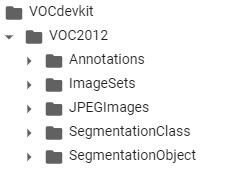
JPEGImages folder contains training images and Annotations folder contains ground truth boxes. Other folders are not necessary for object detection purposes.
Annotations are xml file and contains some unnecessary information. We will define a function parse_annotation that will merge all the annotation files into a single python list discarding unnecessary informations.
def parse_annotation():
    train_data=[]
    for annot_name in sorted(os.listdir(annot_dir)):
        split=annot_name.split('.')
        img_name=split[0]
        img_path=image_dir+img_name
        new_data={ 'object' : [] }
        if os.path.exists(img_path+'.jpg'):
            img_path=img_path+'.jpg'
        elif os.path.exists(img_path+'.JPG'):
            img_path=img_path+'.JPG'
        elif os.path.exists(img_path+'.jpeg'):
            img_path=img_path+'.jpeg'
        elif os.path.exists(img_path+'.png'):
            img_path=img_path+'.png'
        elif os.path.exists(img_path+'.PNG'):
            img_path=img_path+'.PNG'
        else:
            print('image path not exis')

        new_data['image_path']=img_path
        annot=xTree.parse(annot_dir+annot_name)
        for elem in annot.iter():
            if elem.tag == 'width':
                new_data['width']=int(elem.text)
            if elem.tag=='height':
                new_data['height']=int(elem.text)
            if elem.tag=='object':
                obj={}
                for attr in list(elem):
                    if attr.tag=='name':
                        obj['name']=attr.text
                    if attr.tag=='bndbox':
                        for dim in list(attr):
                            obj[dim.tag]=int(round(float(dim.text)))
                new_data['object'].append(obj)
        train_data.append(new_data)
    return train_data
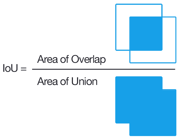
TrainBatchGenerator: This function generates training batch data from the VOC2012 dataset. This function returns two things- training image and ground truth bounding box for three different scales. We calculate IOU between the ground truth box and anchors. IOU is known as Intersection Over Union between two objects. We assume that all anchors and the ground truth box share the same centroid.
If the IOU is greater than 0.3 for any anchor, then we say that this calibration is a positive sample. Using this rule we can generate enough positive samples. But for any gt box, if the IOU is not greater than 0.3, then only the anchor with the largest IOU can be marked as a positive sample. So each gt box gets allocated an anchor box. According to the above principle, a gt box might be matched with multiple anchor boxes.
def preprocess_true_boxes(bboxes):
    label = [np.zeros((output_size[i], output_size[i], anchor_per_scale,
                    5 + num_classes)) for i in range(3)]
    bboxes_xywh = [np.zeros((max_bbox_per_scale, 4)) for _ in range(3)]
    bbox_count = np.zeros((3,))
    for bbox in bboxes:
        bbox_coor = bbox[:4]
        bbox_class_ind = bbox[4]
        onehot = np.zeros(num_classes, dtype=np.float)
        onehot[bbox_class_ind] = 1.0
        uniform_distribution = np.full(num_classes, 1.0 / num_classes)
        deta = 0.01
        smooth_onehot = onehot * (1 - deta) + deta * uniform_distribution
        bbox_xywh = np.concatenate([(bbox_coor[2:] + bbox_coor[:2]) * 0.5, bbox_coor[2:] - bbox_coor[:2]], axis=-1)
        bbox_xywh_scaled = 1.0 * bbox_xywh[np.newaxis, :] / strides[:, np.newaxis]
        iou = []
        exist_positive = False #True means we have found any anchors for gt box
        for i in range(3):
            anchors_xywh = np.zeros((anchor_per_scale, 4))
            anchors_xywh[:, 0:2] = np.floor(bbox_xywh_scaled[i, 0:2]).astype(np.int32) + 0.5
            anchors_xywh[:, 2:4] = anchors[i]
            iou_scale = bbox_iou(bbox_xywh_scaled[i][np.newaxis, :], anchors_xywh)
                                                    #calculates IOU between gt box and anchors
            iou.append(iou_scale)
            iou_mask = iou_scale > 0.3 #IOU_threshold
            if np.any(iou_mask):
                xind, yind = np.floor(bbox_xywh_scaled[i, 0:2]).astype(np.int32)
                label[i][yind, xind, iou_mask, :] = 0
                label[i][yind, xind, iou_mask, 0:4] = bbox_xywh
                label[i][yind, xind, iou_mask, 4:5] = 1.0
                label[i][yind, xind, iou_mask, 5:] = smooth_onehot
                bbox_ind = int(bbox_count[i] % max_bbox_per_scale)
                bboxes_xywh[i][bbox_ind, :4] = bbox_xywh
                bbox_count[i] += 1
                exist_positive = True

        if not exist_positive: # if no anchor having IOU>0.3
            best_anchor_ind = np.argmax(np.array(iou).reshape(-1), axis=-1)
            best_detect = int(best_anchor_ind / anchor_per_scale)
            best_anchor = int(best_anchor_ind % anchor_per_scale)
            xind, yind = np.floor(bbox_xywh_scaled[best_detect, 0:2]).astype(np.int32)
            label[best_detect][yind, xind, best_anchor, :] = 0
            label[best_detect][yind, xind, best_anchor, 0:4] = bbox_xywh
            label[best_detect][yind, xind, best_anchor, 4:5] = 1.0
            label[best_detect][yind, xind, best_anchor, 5:] = smooth_onehot
            bbox_ind = int(bbox_count[best_detect] % max_bbox_per_scale)
            bboxes_xywh[best_detect][bbox_ind, :4] = bbox_xywh
            bbox_count[best_detect] += 1
    label_sbbox, label_mbbox, label_lbbox = label
    sbboxes, mbboxes, lbboxes = bboxes_xywh
    return label_sbbox, label_mbbox, label_lbbox, sbboxes, mbboxes, lbboxes
In the data preprocessing step, we might use data augmentation technique to increase the variety of training set virtually. For example, augmentation includes random color distort, random_horizontal_flip, random_crop, random_translate.
Calculate Loss:
The author regards the target detection task as a regression problem of target area prediction and category prediction. The loss function of YOLOv3 divided into three parts:
- Confidence Loss: To determine whether there are objects in the predicted bounding box. This loss function helps the model to distinguish the background and foreground areas.
- Box Regression Loss: Only applied when the prediction box contains object.
- Classification Loss: To determine which category the object in the prediction box belongs to.
def compute_loss(pred, conv, label, bboxes, i=0, classes=CLASSES):
    NUM_CLASS = len(classes)
    conv_shape  = tf.shape(conv)
    batch_size  = conv_shape[0]
    output_size = conv_shape[1]
    input_size  = STRIDES[i] * output_size
    conv = tf.reshape(conv, (batch_size, output_size, output_size, 3, 5 + NUM_CLASS))

    conv_raw_conf = conv[:, :, :, :, 4:5]
    conv_raw_prob = conv[:, :, :, :, 5:]

    pred_xywh     = pred[:, :, :, :, 0:4]
    pred_conf     = pred[:, :, :, :, 4:5]

    label_xywh    = label[:, :, :, :, 0:4]
    respond_bbox  = label[:, :, :, :, 4:5]
    label_prob    = label[:, :, :, :, 5:]

    giou = tf.expand_dims(bbox_giou(pred_xywh, label_xywh), axis=-1)
    input_size = tf.cast(input_size, tf.float32)

    bbox_loss_scale = 2.0 - 1.0 * label_xywh[:, :, :, :, 2:3] * label_xywh[:, :, :, :, 3:4] / (input_size ** 2)
    giou_loss = respond_bbox * bbox_loss_scale * (1 - giou)

    iou = bbox_iou(pred_xywh[:, :, :, :, np.newaxis, :], bboxes[:, np.newaxis, np.newaxis, np.newaxis, :, :])
    # Find the value of IoU with the real box The largest prediction box
    max_iou = tf.expand_dims(tf.reduce_max(iou, axis=-1), axis=-1)

    # If the largest iou is less than the threshold, it is considered that the prediction box contains no objects, then the background box
    respond_bgd = (1.0 - respond_bbox) * tf.cast( max_iou < IOU_LOSS_THRESH, tf.float32 ) #.5

    conf_focal = tf.pow(respond_bbox - pred_conf, 2)

    # Calculate the loss of confidence
    # we hope that if the grid contains objects, then the network output prediction box has a confidence of 1 and 0 when there is no object.
    conf_loss = conf_focal * (
            respond_bbox * tf.nn.sigmoid_cross_entropy_with_logits(labels=respond_bbox, logits=conv_raw_conf)
            +
            respond_bgd * tf.nn.sigmoid_cross_entropy_with_logits(labels=respond_bbox, logits=conv_raw_conf)
    )

    prob_loss = respond_bbox * tf.nn.sigmoid_cross_entropy_with_logits(labels=label_prob, logits=conv_raw_prob)

    giou_loss = tf.reduce_mean(tf.reduce_sum(giou_loss, axis=[1,2,3,4]))
    conf_loss = tf.reduce_mean(tf.reduce_sum(conf_loss, axis=[1,2,3,4]))
    prob_loss = tf.reduce_mean(tf.reduce_sum(prob_loss, axis=[1,2,3,4]))

    return giou_loss, conf_loss, prob_loss
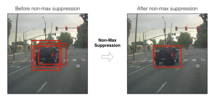
Non-Maximum Suppression:
It is very common in YOLOv3 that multiple bounding boxes predict the same object. So we need to keep the one with highest confidence score and eliminate other bounding boxes with a high overlap rate and low score. This technique is called NMS.
This technique works in three steps:
Step 1: Determine whether the number of bounding boxes is greater than 0 or not. If not, end the process.
Step 2: Select the bounding box with the highest confidence and take it out.
Step 3: Calculate the IOU between the selected bounding box and the remaining bounding boxes. Remove all the bounding boxes whose IOU value is higher than the threshold value. Go to step 1.
We only take all the bounding boxes selected in step 2.
def nms(bboxes, iou_threshold, method='nms'):
    #param bboxes: (xmin, ymin, xmax, ymax, score, class)
    classes_in_img = list(set(bboxes[:, 5]))
    best_bboxes = []

    for cls in classes_in_img: #nms is applied class-wise
        cls_mask = (bboxes[:, 5] == cls)
        cls_bboxes = bboxes[cls_mask]
        # Process 1: Determine whether the number of bounding boxes is greater than 0
        while len(cls_bboxes) > 0:
            # Process 2: Select the bounding box with the highest score according to socre order A
            max_ind = np.argmax(cls_bboxes[:, 4])
            best_bbox = cls_bboxes[max_ind]
            best_bboxes.append(best_bbox)
            cls_bboxes = np.concatenate([cls_bboxes[: max_ind], cls_bboxes[max_ind + 1:]])
            # Process 3: Calculate this bounding box A and
            # Remain all iou of the bounding box and remove those bounding boxes whose iou value is higher than the threshold
            iou = bboxes_iou(best_bbox[np.newaxis, :4], cls_bboxes[:, :4])
            weight = np.ones((len(iou),), dtype=np.float32)
            iou_mask = iou > iou_threshold
            weight[iou_mask] = 0.0

            cls_bboxes[:, 4] = cls_bboxes[:, 4] * weight
            score_mask = cls_bboxes[:, 4] > 0.
            cls_bboxes = cls_bboxes[score_mask]

    return best_bboxes
Training And Testing:
For training and testing code, see YOLOv3.ipynb in this Github repo.