Introduction to K-Nearest Neighbor Classifier

What is KNN:

KNN is the simplest machine learning algorithm which is used in classification and regression problem. KNN stands for k-nearest-neighbor which is a data driven approach where we classify data based on the similarities of sample data. KNN falls in the supervised learning category. Informally, in KNN we are given a dataset(x, y) where x denotes feature and y denotes the class or label. We are interested to learn a function h:X→Y  so that for an unseen observation x, the learned function h(x) can predict the appropriate label y  .

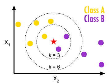
In KNN classification, we assign a label for a new data according to the most common of its k-nearest neighbors. To compute the k-nearest neighbor we need a distance measure function. For numerical valued features, we use Euclidean distance and for categorical or binary valued features we use Hamming distance.

Euclidean distance:

Euclidean distance is also known as the L2 norm. Let x, y are two observations and n is the number of features. Then the Euclidean distance of (x, y) is as follows:

\(dist(x, y)=\sqrt{(x_1-y_1)^2 + ... +(x_n-y_n)^2} \)                            

There are other functions for numerical values such as Manhattan distance, Minkowski distance etc.

Hamming distance:

Hamming distance is used for categorical data. Let x, y are two observations and n is the number of features. Then the hamming distance of (x, y) is as follows:

\(dist(x, y)=\sum_{i=1}^n f(x_i, y_i) \quad \quad, \quad \quad f(x, y)= \begin{cases} 1\quad if \; x\ne y \\ 0\quad if \; x=y \end{cases}\)

Implementation of KNN in python:

In this tutorial, we will use 'Iris.csv' as sample data.

1. Load data from Iris.csv file using panda

import pandas as pd
import numpy as np
import random as random
import matplotlib.pyplot as plt
from sklearn.utils import shuffle

data = pd.read_csv('Iris.csv')
data = data.dropna()              # discarding missing values in data
data = shuffle(data)              # shuffling observations

2. Visualize the data

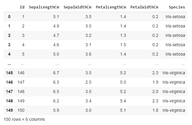
We can see that our ‘Iris.csv’ file contains 150 observations. Each observation consists of 4 features and a label.

Feature: SepalLengthCm, SepalWidthCm, PetalLengthCm, PetalWidthCm

Label: Species

3. Feature scaling

Features scaling is a method to re-scales numerical features of a dataset to a fixed range. A feature has two properties: magnitude and unit

In machine learning algorithm such as KNN, we only care about the magnitude of the features not the unit of the features as we will be using magnitude to calculate distance. So in our dataset, if a particular feature is greater than any other features then the distance function will be biassed towards that feature. Therefore, the range of all features should be in the same range so that they contribute proportionally to the distance function.

There are two methods of feature scaling :

• Normalization: This technique re-scales feature values in between 0 and 1.

\(min-max \: normalization: x^{'} = \frac {x-x_{min}} {x_{max} - x_{min}}\)

• Standardization: This technique re-scales features based on standard normal distribution where mean(μ) is 0 and standard deviation(σ) is 1.

\(x^{'} = \frac {x-\mu} {\sigma}\)

Standardization is more useful when the data follows a Gaussian distribution and the applied algorithm prefers zero centered distribution of data. On the other hand, KNN does not assume any data distribution and our iris dataset does not follow Gaussian distribution. So in this blog we will use normalization for feature scaling. Regardless of these circumstances, we can use any of these two methods of feature scaling as their effect on machine learning algorithm is quite same.

Let’s re-scale features using min-max normalization. We will use scikit-learn object MinMaxScaler for min-max normalization.
 

from sklearn.preprocessing import MinMaxScaler

scaler = MinMaxScaler()

# extracting first 4 columns as features and the last column as label
features = data[['SepalLengthCm', 'SepalWidthCm', 'PetalLengthCm', 'PetalWidthCm']]
labels = data['Species']

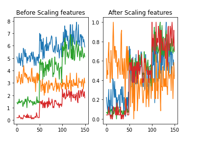
plt.subplot(1, 2, 1)
plt.plot(features)
plt.title("Before Scaling features")

features = scaler.fit_transform(features)
plt.subplot(1, 2, 2)
plt.plot(features)
plt.title("After Scaling features")

4. Distribute the data between the training set and test set

We will split the data set to make training data and test data. Our model will simply store training data and for every test data, we will try to evaluate the appropriate labels. 80% (out of 150 observations) of our data set will be used as training data and the rest of the data set will be used as test data.

num_train = 120                                 # number of training set
num_test = 30                                   # number of test set
num_feature = features.shape[1]                 # number of features per observation
X_train = np.array(features[:num_train])        # (0, 119)'th rows are training data
X_test = np.array(features[num_train:])         # (120, 149)'th rows are test data
Y_train = np.array(labels[:num_train])          # (0, 119)'th rows are training labels
Y_test = np.array(labels[num_train:])           # (120, 149)'th rows are test labels

5. Evaluate predicted labels

To predict label for a test data, we will compute Euclidean distance between the test data and training data. Let’s define a function that will take a single test data and training data and returns the Euclidean distance.

def euclidean_dist(x, y):              # test data, X_train[i]
    dist = 0.0                         # initialize dist variable
    for k in range(num_feature):       # iterate over features
        dist += np.square(x[k]-y[k])   # summation of (x[i]-y[i])^2
    return np.sqrt(dist)               # L2 norm

We’ll iterate over test data and training data using a nested for-loop to calculate distances and store the values in a 2d-array.

\(dists[i, j]= euclidean\_dist(test\_data[i], training\_data[j])\)

Then sort the values and take the indices of K closest distance for every test data. If the problem is a regression problem, we will have to calculate the mean of K labels. For the classification problem, we will have to return the most frequent label of the K labels. As we are classifying the species of iris flower, this problem is a classification problem. Therefore to find the most frequent label from the chosen indices, we’ll use python Counter.

import time
from collections import Counter

def knn(X_test, X_train, Y_train, K):
    pred_y = []                                   # contains the predicted labels
    dists = np.zeros((num_test, num_train))       # 2d array to contains distances
    for i in range(num_test):
        for j in range(num_train):
            dists[i, j] = euclidean_dist(X_test[i], X_train[j])
            
    index = np.argsort(dists, axis=1)             # sort horizontally and 
                                                  # returns indices of sorted array
    for i in range(num_test):
        closest_k = index[i][:K]                  # choose first k'th indices
        count = Counter(Y_train[closest_k])       # contains data pairwise(label, frequency)
        pred_y.append(count.most_common(1)[0][0]) # returns the most frequent label
    return pred_y
        
K = 8
start_time = time.time()
predicted_labels = knn(X_test, X_train, Y_train, K)
end_time = time.time()
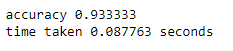
correct_labels = np.sum(predicted_labels == Y_test)

print('accuracy %f' %(correct_labels/num_test))
print('time taken %f seconds' %(end_time-start_time))

Let we have m test data, n training data and d  is the number of features of data.

The time complexity of Euclidean_dist is O(d) as we iterate every feature and for a single test data, we compute distance with every training data. So the time complexity for a test data to compute n distances is O(n*d).

Then we sort the n distances with O(n*logn) complexity and the selection of first K indices from the sorted array is O(K).

So the overall time complexity of KNN for a single test data is O(n*d+n*logn+K).

If we select K  indices from the unsorted array of distances, then the overall time complexity will be O(n*d+n*K).

We can also use the NumPy Linear Algebra function norm to calculate Euclidean distance.

In our KNN code, we use nested for-loop to calculate distances which is not a very good approach. We can use python vectorized implementation as it is quite fast.

Let x and y are two vectors. Then the L2 norm of x and y can be expressed as

\(dist(x, y)=\sqrt{ (x-y)^2 } = \sqrt{ (x^2 + y^2 - 2xy) }\)

Now we have to use this formula in the matrix. The first two parts of the formula can be derived as the L2 norm of every row of X_test and X_train. The last part can be expressed as the dot product of X_test  and transpose of X_train matrices. As the expression is quite complex, we should pay attention to the dimension of the L2  norm and dot product. We’ll use the rehape function to fix the dimension.

import time
from collections import Counter

def knn_vectorized(X_test, X_train, Y_train, K):
    num_test = X_test.shape[0]
    num_train = X_train.shape[0]
    dists = np.zeros((num_test, num_train))
    
    #this is the vectorized implementation
    part_1 = np.sum(X_test**2, axis=1).reshape(num_test, 1)   # x^2
    part_2 = np.sum(X_train**2, axis=1)                       # y^2
    part_3 = 2*X_test.dot(X_train.T)                          # 2xy
    dists = np.sqrt(np.maximum(0, part_1+part_2-part_3))
    
    idx = np.argsort(dists, axis=1)
    pred_y = []
    for i in range(num_test):
        closest = idx[i][:K]
        count = Counter(Y_train[closest])
        pred_y.append(count.most_common(1)[0][0])
    return pred_y
    
K = 8
start_time = time.time()    
predicted_labels = knn_vectorized(X_test, X_train, Y_train, K)
end_time = time.time()
correct_labels = np.sum(predicted_labels == Y_test)

print('accuracy %f' %(correct_labels/num_test))
print('knn_vectorized took %f seconds' %(end_time-start_time))

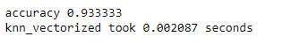
You can see that vectorized implementation is much faster than normal implementation using loops although the time complexity is almost the same. Check the link to understand why vectorized implementation works faster.

6. How to choose Hyperparameter K

We should choose the hyperparameter K that gives us the lowest error. We can run the KNN algorithm for different K and measure the accuracies to choose the appropriate K. In this process, we are using our test data to tune hyperparameter K which is called overfitting as we are forcing our dataset to fit for the test data. So our model will fail in generalizing for new test data. To overcome this problem, we can use a technique called Cross validation. 

In cross validation, we split our training set into k different subset (where this k is different from hyperparameter K). So this is called k-folds cross validation.

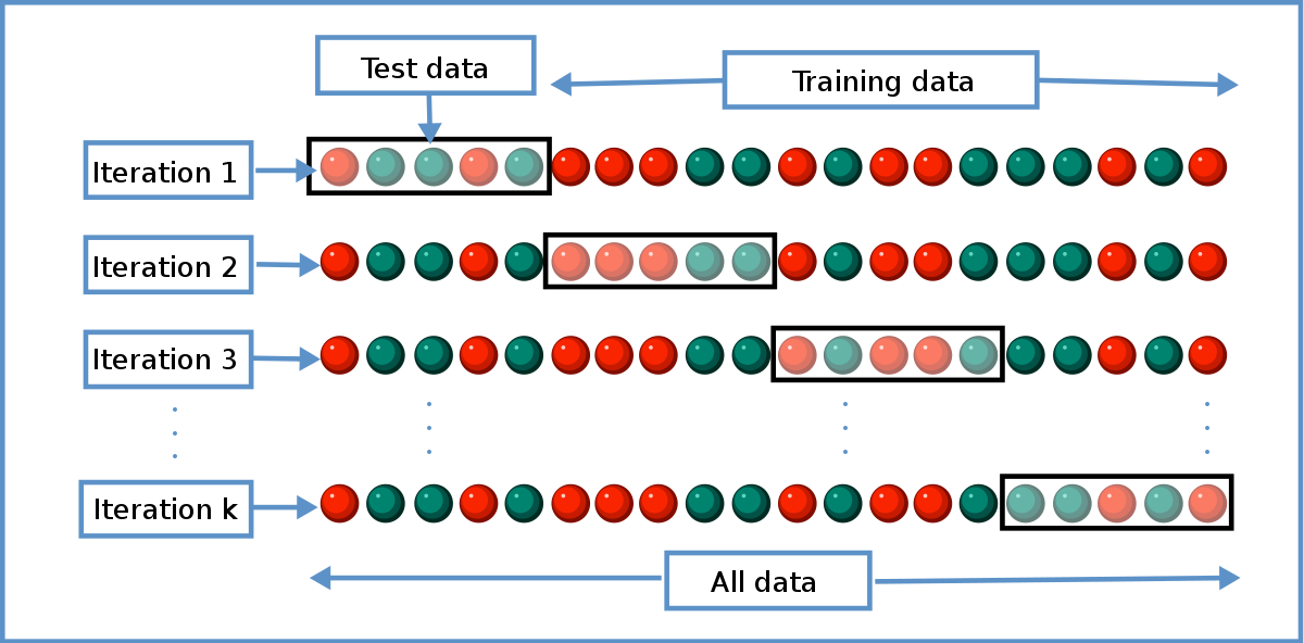
In iteration i, we will choose the i^th subset as our validation data and the remaining subsets as our new training data. We will run our model for different hyperparameter K and will measure accuracy for validation data.

After k iterations, we will choose the hyperparameter K as the best_K whose average accuracy is largest. Here is the code for cross validation.

num_folds = 4
list_of_K = range(1, 80)
X_train_folds = np.split(X_train, num_folds, axis=0)     # spliting X_train
Y_train_folds = np.split(Y_train, num_folds, axis=0)     # spliting Y_train

best_K = 1
best_acc = -1
avg_accuracies = []
for K in list_of_K:
    accuracies = []                                      # contains accuracies for a certain 'K'
    for i in range(num_folds):
        New_X_train = np.concatenate(X_train_folds[: i]+X_train_folds[i+1:]) 
        New_Y_train = np.concatenate(Y_train_folds[: i]+Y_train_folds[i+1:])
        pred_labels = knn_vectorized(X_train_folds[i], New_X_train, New_Y_train, K)
        accuracy = np.sum(pred_labels==Y_train_folds[i]) / X_train_folds[i].shape[0]
        accuracies.append(accuracy)

    avg_acc = np.mean(accuracies)                        # average accuracy for a certain 'K'
    avg_accuracies.append(avg_acc)
    if avg_acc > best_acc:
        best_acc = avg_acc
        best_K = K

print('Best accuracy = %f when K = %d' %(best_acc, best_K))
plt.plot(avg_accuracies)
plt.xlabel('hyperparameter K')
plt.ylabel('accuracy')

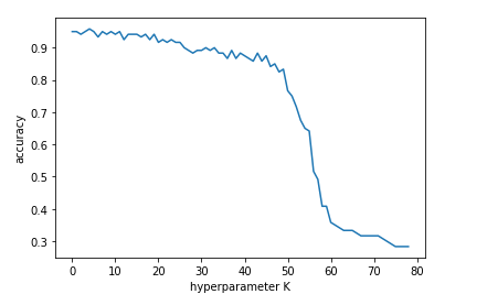
We may expect that our test data will work slightly better if the hyperparameter K=5 . Now run the KNN on test data and see what happens!

import time
from collections import Counter
def knn_vectorized(X_test, X_train, Y_train, K):
    num_test=X_test.shape[0]
    num_train=X_train.shape[0]
    dists=np.zeros((num_test, num_train))
    
    #this is the vectorized implementation
    part_1=np.sum(X_test**2, axis=1).reshape(num_test, 1) #x^2
    part_2=np.sum(X_train**2, axis=1)                     #y^2
    part_3=2*X_test.dot(X_train.T)                        #2xy
    dists=np.sqrt(np.maximum(0, part_1+part_2-part_3))
    
    idx=np.argsort(dists, axis=1)
    pred_y=[]
    for i in range(num_test):
        closest=idx[i][: K]
        count=Counter(Y_train[closest])
        pred_y.append(count.most_common(1)[0][0])
    return pred_y
    
K = 5
start_time = time.time()    
predicted_labels = knn_vectorized(X_test, X_train, Y_train, K)
end_time = time.time()
correct_labels = np.sum(predicted_labels == Y_test)

print('accuracy %f' %(correct_labels/num_test))
print('knn_vectorized took %f seconds' %(end_time-start_time))

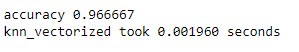
YESSS!!! Accuracy increased by about 3%.