Gradient Descent in Machine Learning

What is Gradient Descent:

Gradient descent is an optimization algorithm. This algorithm is not only used in machine learning but also in various fields of science where optimization or minimizing the value of a function are the ultimate goals. In this blog, we'll see how gradient descent helps us to minimize cost function in various machine learning algorithms. Before diving into gradient descent, let’s discuss minima.

Minima is the plural form of minimum. Minima are of two kinds:

Local minimum: Local minimum is a point of a function where the value of the function is relatively smallest within a certain neighborhood. That means a single function can have multiple local minimum. So the local minimum may not give the smallest value if we consider the whole function.

Global minimum: Global minimum refers to that point of a function where the functional value is the smallest for the whole function.

See the below image for a better understanding of what is local and global minimum.

Let f is a function and θ₁, θ₂, ..., θ_n are the parameters of f, the gradient descent will iteratively find a new set of parameters θ₁^', θ₂^', ..., θ_n^' that minimizes the function which refers to the minima of f. Gradient descent tends to converge at global minimum but it does not guarantee to converge at global minimum all the times. Sometimes gradient descent converges at local minimum.

In machine learning algorithms, we use some observations to train our model so that it can predict appropriate labels/output for new unseen observations. In order to predict output, we use a hypothesis. Hypothesis is a function whose parameters are to be learnt. We initialize the parameters of the hypothesis arbitrarily. Then we calculate loss/error by checking the actual output and the predicted output of the hypothesis. If the loss is high, it refers that our hypothesis is not good enough to predict outputs. So we need to minimize the loss. Here comes the gradient descent. Gradient descent will try to find the global minima of the hypothesis function so that the loss is also minimum. Next we will see how gradient descent actually converges at minima.

How does Gradient Descent work:

Suppose you are hiking in the mountain and want to reach the lowest point of the mountain. Surprisingly you are blindfolded so you cannot see anything. Can you reach the lowest point where there is a lake?

Yes, if you are smart and know about gradient descent. You can take a step in four directions (left, right, ahead, behind) and determine at which direction the land tends to descent. You should repeat this process again and again until you reach a point where you can not find any descending land. This land should be the lowest point where you wanted to go. Gradient descent works on the same method.

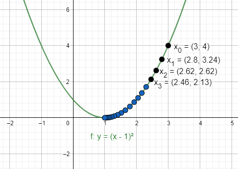
Suppose  \(y=(x-1)^2\) is our loss function that is to be minimized. Gradient descent will choose a random point, let \(x_0=3\)  and learning rate \(lr = 0.05\). If we want to relate this to our previous mountain example, we would say that \(x_0 = \) peak point of the mountain, \(lr = \) the size of step we take towards the descending land.

The gradient of the loss function is \({dy\over{dx}} = 2*(x-1) \)          where  \({dy\over{dx}}= \begin{cases} >0 \quad\quad ascending \; land \\ <0 \quad\quad descending \; land \\ =0 \quad\quad flat \; land \end{cases}\)

Now we start to iterate.

\(x_1 = x_0 - lr * {dy \over{dx}} = 3 - 0.05 * 2 * (3-1) = 2.8\)

\(x_2 = x_1 - lr * {dy \over{dx}} = 2.8 - 0.05 * 2 * (2.8-1) = 2.62\)

     \(x_3 = x_2 - lr * {dy \over{dx}} = 2.62 - 0.05 * 2 * (2.62-1) = 2.46\)

\(​​​​...\quad...\quad...\)

\(​​​​...\quad...\quad...\)

 

After a few steps, we will reach \((1, 0)\) where the loss is 0 which is the minimum loss for our function. 

Few things about gradient descent:

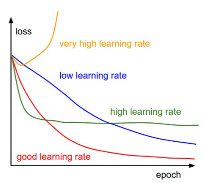
• The learning rate in gradient descent is a hyperparameter which is often in the range between \(0.001\) and \(0.1\) . Learning rate indicates how fast we want to converge at minima. If the learning rate is too small then our model will take forever to converge. If the learning rate is too big then our model will be unstable and our model may not converge at minima at all. So we have to choose the learning rate carefully.

• Gradient descent starts to converge rapidly at the beginning but after a few iterations, it converges quite slowly. Because at the beginning our initial point lies far from the minima point and at that point, the gradient is quite large. After a few successive iterations, our initial point gets closer to minima and at that point, the gradient is smaller than the previous point. As our initial point gets closer to minima, the gradient gradually shrinks.
• At the minimum point, the gradient is zero. So we can terminate gradient descent algorithm when we converge at minimum point by checking the gradient. In most of the real-life problems, we can not converge at the actual minimum point but our point may be very close to the minimum point. So we can fix the number of iterations.

 

Linear Regression: 

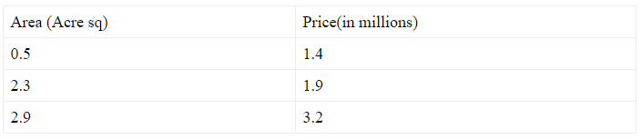
Linear regression is a supervised machine learning algorithm. It predicts output \((y)\) based on the linear relationship of one or many independent variables \((x)\). These independent variables are called input features and the dependent variable is called output target. Let’s build a simple linear regression model for housing prices dataset. For the sake of simplicity, we will use a very short dataset for our model.

Now define some notations for future use.

\(x^i\)= independent variables(living area in this example). Here superscript \((i)\) refers to the i'th training set.

\(y^i \)= dependent variable(price in this example). Here superscript \((i)\) refers to the i'th training set.

\(m\)= number of training examples. In this example \(m=3\)

\(n\)= number of independent variables in each training set. In this example, we have one independent variable(living area). So \(n=1\)

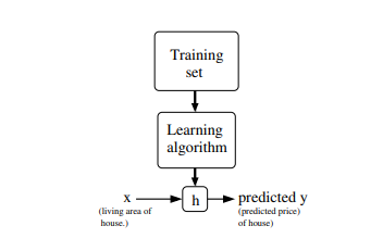
In linear regression algorithm, our goal is to learn a function \(h\) that takes training set features as input and predicts the corresponding output target. Historically we call this function a hypothesis. So linear regression algorithm works like this(see below picture).

Now we need to define our hypothesis to perform linear regression. \(h_{\theta}(x)= \sum_{i=0}^{n} x_i \theta_i\) ,   where  \(x_0=1\)

 

Here \(\theta_i\) are the parameters of the hypothesis \(h\) that we need to learn to make \(h_{\theta}(x^i)\) close to \(y^i\). So we need a function that can measure how close the value of \(h_{\theta}(x^i)\) to its actual target \(y^i\). we call this loss/cost function.

\(J(\theta)=\frac{1}{2m}\sum_{i=1}^{m}(h_{\theta}(x^i)-y^i)^2\)

This loss function is called MSE mean squared error.

Now we have a hypothesis to predict the target and a loss function to compute the error between the actual target and the predicted target. But how can we minimize the error? Here comes the gradient descent. We will use gradient descent on loss function to learn the \(\theta_i\) and therefore minimize the error.

 \(\theta_j := \theta_j - \alpha \frac{\partial}{\partial \theta_j} J(\theta)\)

\(\frac{\partial}{\partial \theta_j} J(\theta)= \frac{\partial}{\partial \theta_j} (\frac{1}{2m} \sum_{i=1}^{m}(h_\theta(x^i)-y^i)^2)\)

\(\frac{\partial}{\partial \theta_j} J(\theta)= \frac{1}{2m}*2 \sum_{i=1}^{m}(h_{\theta}(x^i)-y^i) \frac{\partial}{\partial \theta_j}(h_{\theta}(x^i)-y^i)\)

\(\frac{\partial}{\partial \theta_j} J(\theta)= \frac{1}{m} \sum_{i=1}^{m}(h_{\theta}(x^i)-y^i) \frac{\partial}{\partial \theta_j}(x_0^i \theta_0^i + ...+x_j^i\theta_j^i + ... +x_n^i\theta_n^i - y^i)\)

\(\frac{\partial}{\partial \theta_j} J(\theta)= \frac{1}{m} \sum_{i=1}^{m} (h_{\theta}(x^i)-y^i)x_j^i\)

\(So \quad \theta_j := \theta_j - \alpha \frac{1}{m} \sum_{i=1}^{m}(h_{\theta}(x^i)-y^i)x_j^i\)

 

Now let's plot our data. For the sake of simplicity, we will use constant value of \(\theta_0=0\) which means our hypothesis passes through \((0, 0)\) and the learning rate \(\alpha = 0.1 \). So \(h_{\theta}(x)=\theta_1x_1\)

Initialize \(\theta_1=1\) and plot the hypothesis.

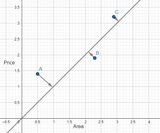
 \(\frac{\partial}{\partial \theta_j} J(\theta)=\frac{1}{3}((1.0*0.5-1.4)*0.5 +(1.0*2.3-1.9)*2.3 +(1.0*2.9-3.2)*2.9 ) \\ \quad \quad \quad =-0.4 \\ Update \quad \theta_1, \quad \quad \theta_1= \theta_1 - \alpha * \frac{\partial}{\partial \theta_j}J(\theta) = 1.0 - 0.1*(-0.4) = 1.04\)

Plot the hypothesis again for \(\theta_1 = 1.04\)

 

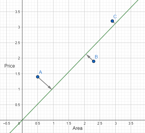
\(\frac{\partial}{\partial \theta_j} J(\theta)=\frac{1}{3}((1.04*0.5-1.4)*0.5 +(1.04*2.3-1.9)*2.3 +(1.04*2.9-3.2)*2.9 ) \\ \quad \quad \quad =0.0527 \\ Update \quad \theta_1, \quad \quad \theta_1= \theta_1 - \alpha * \frac{\partial}{\partial \theta_j}J(\theta) = 1.04 - 0.1*(0.0527) = 1.035\)

After a few iterations, we will get our desired optimal \(\theta_1\)

 

Types of Gradient Descent:

• Batch Gradient Descent: This type of gradient descent processes the whole dataset for every iteration. Though batch gradient descent converges quickly in terms of iterations, it is computationally very expensive. So this is not preferred for large datasets. If the dataset is quite small, then we should use batch gradient descent. Here is the update method for batch gradient descent:

\(\theta_j := \theta_j - \alpha \frac{1}{m} \sum_{i=1}^{m}(h_{\theta}(x^i)-y^i)x_j^i\)

 

• Stochastic Gradient Descent: To make the update operation faster, we use single training example in every iteration. As we are using single training example instead of whole dataset, we need a lot of iterations to converge at global minima. Although stochastic gradient descent needs a lot of iterations, it is still faster than batch gradient descent for large datasets. Here is the update method for stochastic gradient descent:         

\(\theta_j := \theta_j - \alpha (h_{\theta}(x^k)-y^k)x_j^k\)

 

• Mini Batch Gradient Descent: In batch gradient descent, we need a few iterations but the iterations are quite expensive and in stochastic gradient descent, the iterations are quite fast but we need a lot of iterations. Mini batch gradient descent works faster than both batch and stochastic gradient descent. This is a kind of trade-off between batch gradient descent and stochastic gradient descent. In mini batch gradient descent, we divide dataset into some small batches. For every iteration, we process single batches. Therefore we do not need a lot of iteration and the iterations are also not very expensive as batch gradient descent. Here is the update method for mini batch gradient descent:

\(\theta_j := \theta_j - \alpha \frac{1}{k} \sum_{i=1}^{k}(h_{\theta}(x^i)-y^i)x_j^i \quad \quad where \quad k=batch \quad size \quad of \quad dataset\)