Generative Adversarial Networks(GANs) part 1
Author: Sadekujjaman Saju
Created: 28 Jun, 2021
Last Updated: 02 Nov, 2024
Last Updated: 02 Nov, 2024
Generative adversarial networks (GANs) are the most exciting recent innovation in the machine learning area. Generative Adversarial Networks, A deep learning method such as convolutional neural networks, an approach to generative modeling: creates new sample data instances that resemble training data. GANs can create images that look like photographs of human faces, even though the faces don't belong to any real person.
In this tutorial, we will discuss very basic learning materials for GANs.
Table of contents
Machine Learning
Supervised Learning
Unsupervised Learning
Reinforcement Learning
Deep Neural Network
Generative modeling
Gaussian Distribution
Dimensionality Reduction
Encoder
Decoder
Latent Space
Autoencoder
Autoencoder and Prism
Variational Autoencoder
Machine Learning
Machine Learning is the study of computer algorithms or a method of data analysis that makes the computer ability to learn. It is a branch of Artificial Intelligence. It automates the analytical model building. Machine Learning is one of the most exciting technologies that would have ever come across. It focuses on the development of computer algorithms that can
-
Learn from data
-
Identify patterns
-
Make predictions with minimal human intervention
-
Improve automatically through experience
We can categorize the most widely adopted machine learning methods as supervised learning, unsupervised learning, and reinforcement learning. We will briefly discuss these in the following tutorial.
Supervised Learning
Supervised Learning is the machine learning task where machines are learned from “labeled data” and predict outcomes for unseen data. It learns a mapping function that maps an input to an output based on training examples. In training, we give both input and output to the function which maps an input to output and adopts to learn for unseen input.
The learning task is called supervised learning because learning from the labeled dataset can be thought of as a teacher supervising the learning process. We know the correct answers, the algorithm iteratively makes predictions on the training data and is corrected by the teacher. Look at the example given below:
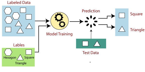
Figure: Working process of supervised learning Image source
Suppose we have a dataset of different types of shapes which includes square, rectangle, triangle, and Polygon. Now the first step is that we need to train the model for each shape.
- If the given shape has four sides, and all the sides are equal, then it will be labeled as a Square.
- If the given shape has three sides, then it will be labeled as a triangle.
- If the given shape has six equal sides, then it will be labeled as a hexagon.
Now, after training, we test our model using the test set, and the task of the model is to identify the shape.
The machine is already trained on all types of shapes, and when it finds a new shape, it classifies the shape based on the number of sides and predicts the output.
Unsupervised Learning
Unsupervised Learning is the machine learning task where machines are learned from “unlabeled data” and learns some pattern from data. In unsupervised learning, we have only input data and the goal is to find the underlying structures or patterns or groups of input data. It can discover similarities and differences in data for making a realistic assumption about data. In unsupervised learning, training examples are not labeled, and finds the patterns without any supervision. Clustering, for example, is an unsupervised learning example—because we are just trying to discover the underlying structure of the data; but anomaly detection is usually supervised, as we need human-labeled anomalies. Look at the example given below:
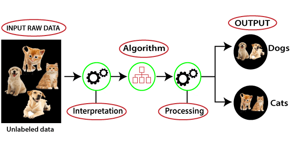
Figure: Working process of unsupervised learning Image Source
Here, we have taken unlabeled input data, which means it is not categorized and corresponding outputs are also not given. Now, this unlabeled input data is fed to the machine learning model to train it. Firstly, it will interpret the raw data to find the hidden patterns from the data and then will apply suitable algorithms such as k-means clustering, Decision tree, etc.
Once it applies the suitable algorithm, the algorithm divides the data objects into groups according to the similarities and differences between the objects.
Reinforcement Learning
Reinforcement Learning (RL) is a sub-area of machine learning techniques that are inspired by natural systems/psychology where we can learn via interaction with the environment. In our daily life, we learn a lot by interacting with the environment. when a child learns to talk or a cat learns to act with us, it has no explicit teacher, but it does have a direct connection to its environment. In fact, whether we are learning to drive a car or to hold a conversation, we are acutely aware of how our environment responds to what we do, and we seek to influence what happens through our behavior.
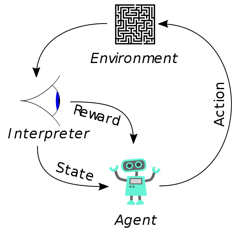
Figure: The typical scenario of Reinforcement Learning
In Reinforcement Learning, there are two fundamental elements. One is Agent and another is Environment. The agent is one who takes action and gets rewards based on their action. And the environment is the Agent's world in which it lives and interacts. So, the agent is the learner and decision-maker in this case and the thing agent interacts with is called the environment.
The agent is rewarded for each action. If the action taken by the agent is good/right, the agent will get a positive reward from the environment. On the other hand, if the action taken is bad/wrong, it will get a negative reward from the environment. The goal of the agent is to maximize rewards.
Now we are going to discuss Deep Neural Network and Generative Modeling which are necessary concepts to know before knowing Generative adversarial network.
Deep Neural Network
The neural network is a series of algorithms that are designed to recognize patterns or underlying relationships in the input data. A neural network is a network made up of biological neurons for solving artificial intelligence (AI) problems. It is a collection of interconnected units or nodes called neurons. Every connection like the synapses in a biological brain can transmit the signal to another connected neuron and these neurons received the transmitted signal and processed it.
The network consists of various layers where each layer has multiple neurons. The neurons or nodes are interconnected to one another in various layers. The first layer is called the input layer and the last layer is called the output layer and the intermediate layer is called the hidden layer. Each neuron performs complex computation and passes the result to connected neurons. Then the output layer transforms the result into the desired output.
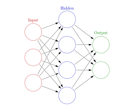
Figure: Basic diagram of neural networks
Generative Modeling
We are familiar with how deep learning takes raw pixels and turns them into, for example, class predictions. For example, we can take three matrixes that contain pixels of an image (one for each color channel) and pass them through a system of transformations to get a single number at the end. But what if we want to go in the opposite direction? What if we want to generate new images instead of predictions? Here comes the idea of generative modeling. A generative model describes how a dataset is generated, in terms of a probabilistic model. By sampling from this model, we are able to generate new sample data. More formally, we take a certain image (real sample) and try to generate new samples from it which look as realistic as the real sample.
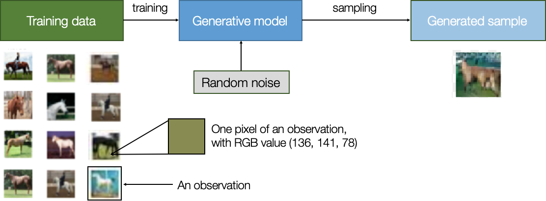
Figure: Process of generative modeling Image source
Autoencoder is an example of generative modeling. Before diving into autoencoder, we will discuss briefly some fundamental topics like encoder, decoder, latent space which are related to it. We also want to discuss two optional materials, Gaussian Distribution and Dimensionality Reduction which might be helpful in the future.
Gaussian Distribution
Gaussian Distribution is also known as normal distribution is a probability distribution used for independent, randomly generated variables. It is often described as a “bell-shaped curve”. Gaussian distribution has two parameters: the mean and the standard deviation. It is symmetric about the mean and showing that data near the mean occur more frequently than data far from the mean. In a normal distribution, the mean is zero and the standard deviation is 1. The general probability density function is given below:
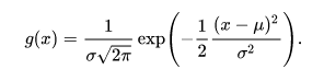
Here, the parameter \(\mu\) is the mean of the distribution while the parameter \(\sigma\) is its standard deviation. The graph of the probability density function is as follows:
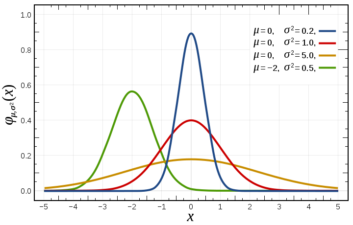
Figure: Probability density function (The red curve is the standard normal distribution) image source
Dimensionality Reduction
In machine learning, the number of input variables or features for a dataset is referred to as its dimensionality. The more features there are, the greater the dimensions of the dataset. In a dataset, the more features have, the more information we have got. If we have high dimensionality in our dataset, the machine learning model can easily extract the information and predict different types of results.
But often the work for the machine learning model becomes complicated if the dataset has too many input features. This can dramatically impact the performance of machine learning algorithms fit on data with many input features. At such times we have to remove some features. Features have to be removed in such a way that the main features of the dataset are not removed. This feature removal process is known as Dimensionality Reduction.
Encoder
An encoder network is a one or many-layer neural network that compresses high-dimensional input data into a lower-dimensional representation vector. We take an input representation x and then a learned encoder reduces the dimension from x1 to x2 where x1 > x2 and generates an output representation z. An encoder network is given below:
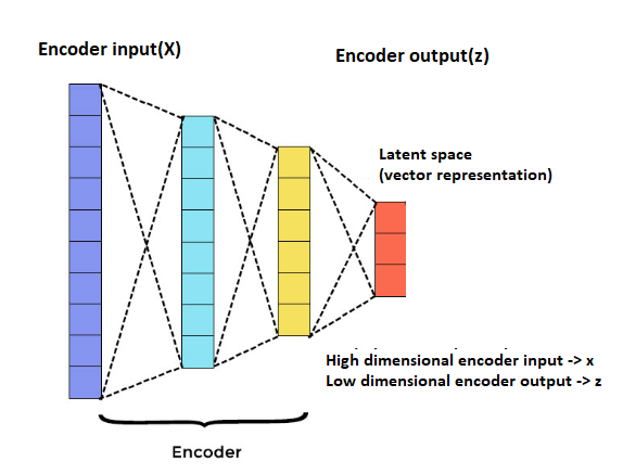
Figure: Encoder Network
Decoder
A decoder network is opposite to an encoder network. It is also a one or many-layer neural network that decompresses a given representation vector back to the original domain. We take a representation z and then a learned decoder enhances the dimension from x2 to x1 where x2 < x1 and produces an output representation x*. A decoder network is given below:
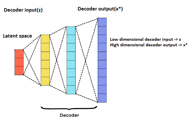
Figure: Decoder Network
Latent Space
Latent space is the hidden representation of compressed data. It is a learned representation, meaningful to people in ways we think of it. In other words, Latent space refers to an abstract multi-dimensional vector space containing feature values that we cannot interpret directly, but which encodes a meaningful internal representation of externally observed events.
Different models will learn a different latent representation of the same data. Typically, it is a 100-dimensional hypersphere with each variable drawn from a Gaussian distribution with a mean of zero and a standard deviation of one.
Let's dive into autoencoder, a generative model.
Autoencoder
Autoencoder is a type of neural network that can be used to learn a compressed representation of raw data. It helps us encode data, well, automatically. It is composed of two parts:
- Encoder
- Decoder
An autoencoder network is given below:
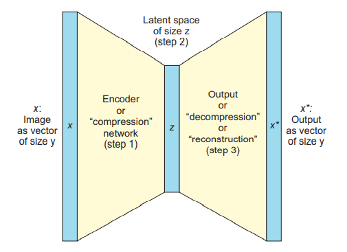
Figure: An Autoencoder network (Encoder and Decoder)
In Autoencoder the encoder compresses the input x and the decoder attempts to recreate the input as x* from the compressed version z provided by the encoder.
More generally, an encoder is a feedforward, fully connected neural network that compresses the input into a latent space representation. For example, an encoder encodes the input image as a compressed representation in a reduced dimension. The compressed image is the distorted version of the original image. The model learns how to reduce the input dimensions and compress the input data into an encoded representation
The Decoder is also a feedforward network like the encoder and has a similar structure to the encoder. This network is responsible for reconstructing the input back to the original dimensions from the compressed representation. The model learns how to reconstruct the data from the encoded representation to be as close to the original input as possible.
Autoencoder and Prism
In optics, some piece of glass cut with a specific shape, useful for analyzing and reflecting light, is called prism. An ordinary prism can separate white light into its constituent colors, called a spectrum. Generally, seven colors or spectrums we can extract from a white light source passing through a prism.
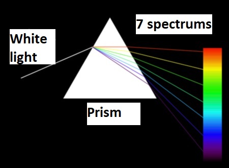
Figure: The white light passing through a prism and divided into 7 spectrums
On the other hand, we can merge these 7 spectrums to get white color. Seven spectrums pass through the prism and the prism combines these spectrums and constructs a white light source.
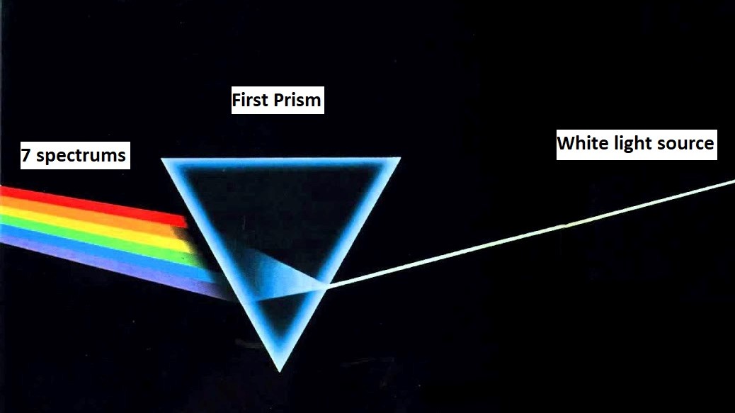
Figure: The seven spectrums passing through a prism and these spectrums are converted into white light
We can also combine these two processes. For this, we place two prisms. After that, we pass seven spectrums through the first prism. The first prism combines these seven spectrums into one white light source. Then the white light source passes through the second prism. The second prism extracts seven spectrums back again.
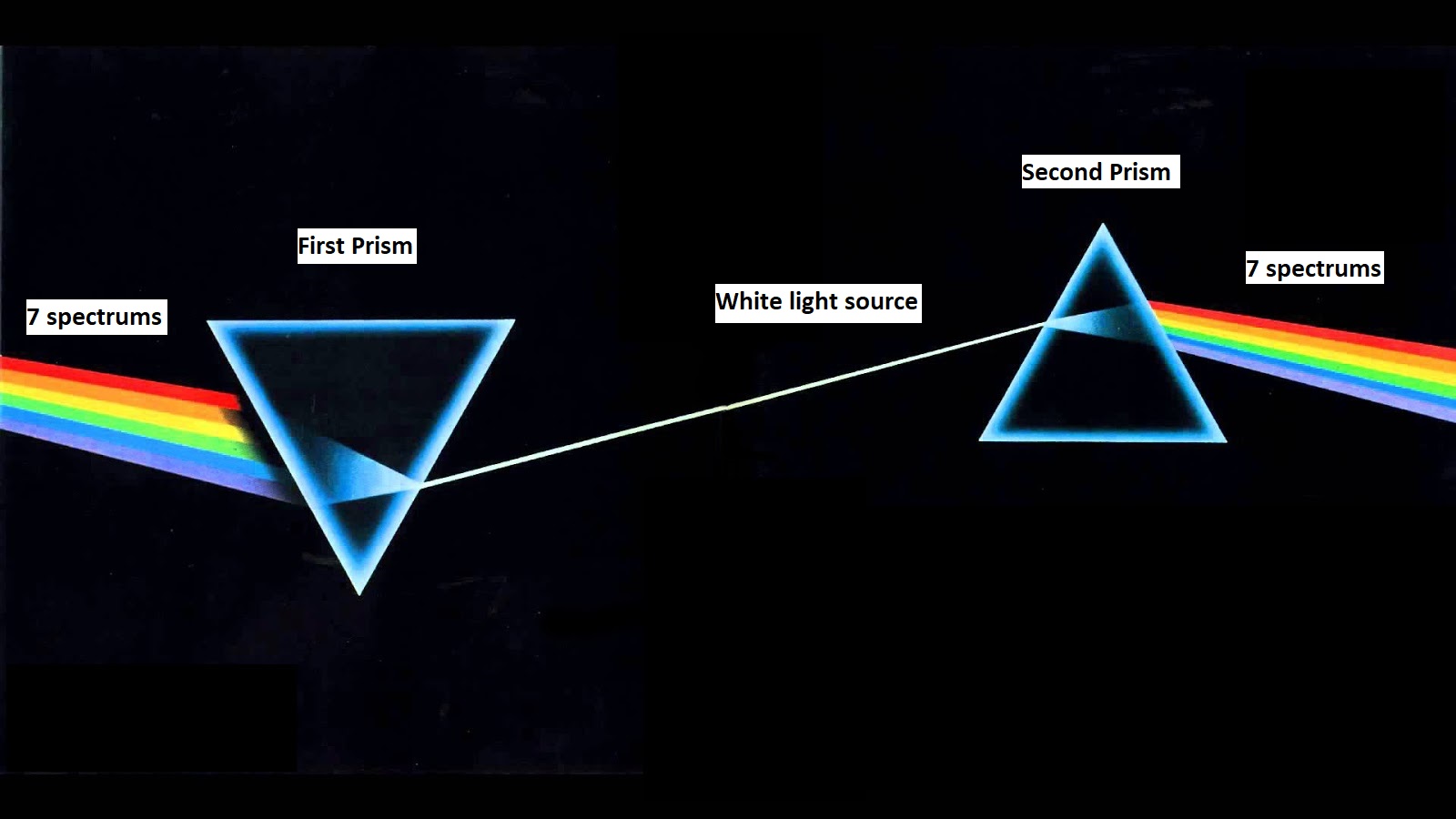
We can divide this prism concept into 3 cases.
-
Extract 7 spectrums from a white light source.
-
Merge 7 spectrums to construct a white light source.
-
Constructing white light source from seven spectrums and then pass this white light to another prism to extract seven spectrums back again
-
We can assume that 7 spectrums input data as 7-dimensional data and white light source as one-dimensional data.
We can think of the prism as a machine learning model, seven spectrums as input data, and a white light source as a compressed representation of input data.
Case 1: We can relate it with decoder, where the compressed representation passes through a machine learning model and then the machine learning model decompresses the representation to original data. If we want to describe it in the machine learning language – A one-dimensional compressed data passes through a machine learning model called a decoder and the decoder produces seven-dimensional (7 spectrums) output data.
Case 2: We can relate it with an encoder, where input data passes through a machine learning model, the machine learning model then converts the input data to a compressed form. In machine learning language – Seven-dimensional input data (7 spectrums) passes through a machine learning model called encoder and the encoder produces one-dimensional (white light) compressed data.
Case 3: We can relate it with autoencoder, where the first prism is encoder (Merges 7 spectrums into a white light source) and the second prism is decoder (Extracts 7 spectrums back from the white light source). In this case, high-dimensional input data (7-dimensional spectrums) passes through a machine learning model called encoder; the encoder produces low dimensional compressed output (one dimensional light source) of the input data. Then the low dimensional compressed output passes through another machine learning model called decoder, the decoder produces high dimensional data (7-dimensional spectrums) back again like input data.
Variational Autoencoder
Variational Autoencoder (VAE) is the artificial neural network model architecture similar to autoencoder. Because of the model architecture of the autoencoder, VAE is often associated with it. But there is a significant number of differences both in the goal and in the mathematical representation. In autoencoder, input data is mapped directly to one point in latent space. In variational autoencoder, input data is instead mapped to a multivariate gaussian distribution. VAE learns probability distribution of data where autoencoder learns a function map to each input to a number and decoder learns the reverse mapping. VAE is a generative autoencoder, they can generate new instances that look similar to original input data. We can see the difference between autoencoder and variational autoencoder in the given picture:
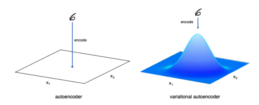
Figure: The difference between autoencoder and variational autoencoder
In the figure given below, VAE the encoder compresses the input x into a latent space. This time encoder tends to produce the result that looks as they were sampled from Gaussian distribution. and the decoder attempts to reconstruct the input.
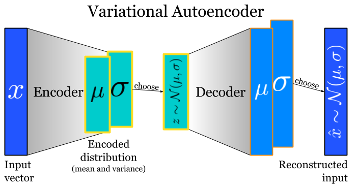
Figure: Variational autoencoder network image source
Next tutorial we will discuss more details about Generative Adversarial Network and its components.